
Results
Three studies are reported here. Two test activity predictions against published cell assay measurements, one for copper complexes and one for ruthenium complexes. The third compares optimised ruthenium structures with crystal structures. All three are retrospective and the datasets are small. The Methods page explains how the tests were run.
Copper activity prediction
The dataset holds 26 copper complexes with IC50 values measured in MCF-7 breast cancer cells. Twenty of them come from five published studies [1–5], and six were added later from five more [6–10].
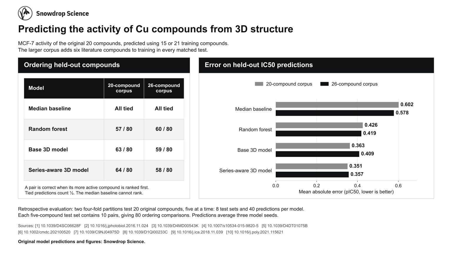
The main test predicts the original 20 complexes. They are divided into four groups of five, and each group is predicted by models trained on the other 15. This is done for two different divisions, so each complex is predicted twice, both times by models that were not trained on it. The test is then repeated with the six added complexes included in training, which gives 21 training compounds for the same held-out groups.
Four methods are compared. The median baseline predicts the median pIC50 of the training compounds for every complex. The random forest [11] is trained on summary descriptors of each complex. The two 3D models take the 3D structure as input. The base model is trained on the activity of each compound, and the series-aware model is also trained on the activity differences between related compounds in the training set.
| Method | 15 training compounds | 21 training compounds | ||
|---|---|---|---|---|
| MAE | Correct pairs | MAE | Correct pairs | |
| Median baseline | 0.602 | n/a | 0.578 | n/a |
| Random forest | 0.426 | 57 | 0.419 | 60 |
| Base 3D model | 0.363 | 63 | 0.409 | 59 |
| Series-aware 3D model | 0.351 | 64 | 0.357 | 58 |
A pIC50 value is 6 minus the base-10 logarithm of the IC50 in µM, so an MAE of 0.351 means that the predicted and measured IC50 values differ by a factor of about 2.25 on average.
With 15 training compounds, the series-aware 3D model had the lowest error, 0.351, and ordered 64 of the 80 pairs correctly. Adding the six complexes to training did not help the 3D models. The error of the base model rose from 0.363 to 0.409, and both 3D models ordered fewer pairs correctly, slightly fewer than the random forest. The six added complexes differ from the original 20 in both ligand type and laboratory of origin, so this test cannot tell which of the two caused the change.
Predicting beyond the training range
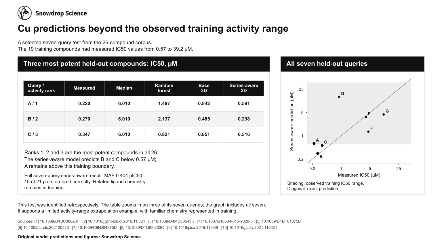
A harder test is to predict complexes that are more potent than any compound in the training set. In one division of the 26-compound dataset, the seven held-out complexes included the three most potent of all 26. The 19 training compounds had IC50 values from 0.57 to 39.2 µM. The series-aware model predicted two of the three below 0.57 µM. Its predictions were 0.298 and 0.516 µM against measured values of 0.270 and 0.347 µM. It predicted the most potent complex at 0.591 µM against a measured 0.220 µM. Complexes from the same ligand family remained in the training set.
Over all seven held-out complexes, the series-aware model had an MAE of 0.404 and ordered 15 of 21 pairs correctly. The random forest ordered 17 of 21. One complex with a measured IC50 of 0.90 µM was predicted at 14.6 µM. This division was picked out after its results were known, so it shows what the model did in one case and says nothing about how often it would do so.
Limits at the ends of the range
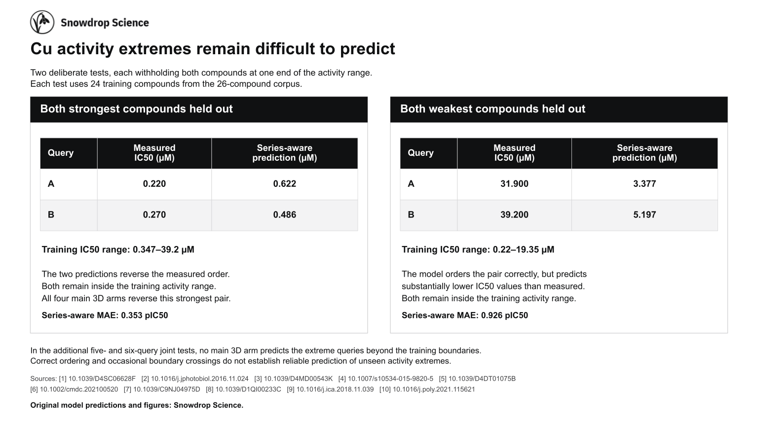
Two further tests each held out both complexes at one end of the activity range and trained on the other 24. With the two most potent complexes held out, the series-aware model predicted 0.622 and 0.486 µM against measured values of 0.220 and 0.270 µM. Both predictions stayed inside the training range, and their order was reversed. The base 3D model reversed the pair as well, as did both models when trained on the 20-compound dataset. With the two least potent complexes held out, the series-aware model ordered them correctly but predicted 3.38 and 5.20 µM against measured values of 31.9 and 39.2 µM. Its MAE in that test was 0.926, slightly worse than the median baseline at 0.887.
Two more tests held out five and six complexes taken from both ends of the range. In those, neither 3D model predicted the most and least potent complexes beyond the limits of its training data.
In the main test the 3D models had lower errors than both baselines. Their lead in ordering pairs was lost when the six added complexes were included in training, and none of these tests shows reliable prediction beyond the range of the training data.
The three figures are also available as one PDF. The IC50 values are the work of the authors of the ten cited studies. The predictions and figures are by Snowdrop Science.
Ruthenium activity prediction
The ruthenium dataset holds 49 ruthenium(II) arene complexes tested against A2780 ovarian cancer cells in two studies that used the same growth inhibition assay [12, 13]. An IC50 value was reported for 31 of them. For the other 18 only a limit was reported, such as an IC50 above 100 µM, and those complexes are left out of the errors in Table 2.
The dataset was divided into groups at random in three different ways. For each way, every group was held out in turn and predicted by a model trained on the rest. The same was done for a fourth division that was fixed during earlier work.
| Method | Mean of three random divisions | Lowest and highest of the three | Earlier division |
|---|---|---|---|
| Mean baseline | 0.422 | 0.407 to 0.442 | 0.408 |
| Random forest | 0.405 | 0.391 to 0.431 | 0.369 |
| 3D model | 0.362 | 0.333 to 0.395 | 0.368 |
| 3D model with electronic properties | 0.330 | 0.317 to 0.347 | 0.384 |
The mean baseline predicts the mean pIC50 of the training compounds, and the random forest [11] is trained on summary descriptors of each complex. The 3D model takes the 3D structure as input. The last model is also given computed electronic properties of each complex.
Of these four methods, the 3D model with electronic properties had the lowest error on each of the three random divisions. On the earlier division the order changed. The 3D model without electronic properties and the random forest were level at 0.368 and 0.369, and the model with electronic properties was behind them at 0.384. All four divisions score the same 31 complexes, so the differences between them show how much the result depends on the division. They do not count as repeat experiments.
The copper and ruthenium results come from different cell lines and assays. Their errors cannot be compared with each other, and they say nothing about which metal gives the more active compounds.
Geometry optimisation compared with crystal structures
Thirteen ruthenium(II) arene complexes with published crystal structures [13, 14] were optimised with GFN2-xTB in implicit water [15, 16], without restraints, starting from their crystal coordinates. Table 3 compares each optimised structure with its crystal structure. Because every optimisation started from the crystal structure, the table shows how far GFN2-xTB moves a complex away from experiment. Predicting a crystal structure from a structure built by hand is a separate test, and it is not part of this study.
| Complex | CCDC | Arene | Chelating ligand | RMSD | Ru to arene centroid | Ru–N | Ru–Cl |
|---|---|---|---|---|---|---|---|
| RM175 | 170362 | biphenyl | ethylenediamine | 0.161 | 0.131 | 0.008 | 0.022 |
| 16 | 607563 | fluorene | ethylenediamine | 0.117 | 0.123 | 0.006 | 0.028 |
| 22 | 607565 | tetralin | ethylenediamine | 0.123 | 0.116 | 0.003 | 0.024 |
| 27 | 607573 | indan | 1,3-diamino-2-propanol | 0.100 | 0.140 | 0.016 | 0.014 |
| 28 | 607562 | indan | homopiperazine | 0.080 | 0.147 | 0.024 | 0.032 |
| 36 | 607564 | tetrahydroanthracene | 1,2-diaminobenzene | 0.506 | 0.129 | 0.021 | 0.004 |
| 38 | 607570 | indan | 2,2′-bipyridine | 0.083 | 0.189 | 0.106 | 0.029 |
| 39 | 607572 | biphenyl | 2,2′-bipyridine | 0.122 | 0.157 | 0.095 | 0.014 |
| 43 | 607571 | indan | 1,10-phenanthroline | 0.072 | 0.177 | 0.089 | 0.035 |
| 53 | 607567 | p-cymene | 8-hydroxyquinolinate | 0.176 | 0.158 | 0.085 | 0.022 |
| 60 | 607574 | p-cymene | 2,2,6,6- | 0.354 | 0.179 | n/a | 0.021 |
| 61 | 607566 | p-cymene | hexafluoroacetylacetonate | 0.464 | 0.203 | n/a | 0.042 |
| 62 | 607568 | p-cymene | chromenone diketonate | 0.580 | 0.187 | n/a | 0.019 |
All 13 optimisations converged with no bonds broken or formed. The median differences were 0.023 Å for Ru–N bonds in the 10 complexes with nitrogen donors, 0.022 Å for Ru–Cl bonds and 0.68° for the chelate bite angle. The median heavy-atom RMSD was 0.12 Å.
Two differences are systematic. GFN2-xTB placed ruthenium on average 0.16 Å further from the arene centroid than in the crystal structures, and it shortened bonds to aromatic nitrogen donors by 0.085 to 0.106 Å. In the four complexes with the largest RMSD, 0.35 to 0.58 Å, the Ru–Cl differences are still at most 0.042 Å. Their RMSD comes from the orientation of fused rings and ligand substituents. The crystal structures are solids that include counter-ions, while the calculations model a single complex in implicit water.
RM175 compared with density functional theory
RM175, [(η6-biphenyl)Ru(en)Cl]+, was also optimised with density functional theory, using the ωB97M-V functional [18], the def2-SVP basis set [19] with an effective core potential for ruthenium [20] and the SMD water model [21]. The calculation ran on a cloud GPU with PySCF and GPU4PySCF [22, 23]. A vibrational frequency calculation supports a local minimum. Table 4 compares RM175 at each stage with its crystal structure [24].
| Structure | Ru–Cl | Ru–N | Mean Ru–C | Ru height above arene | N–Ru–N | RMSD to crystal |
|---|---|---|---|---|---|---|
| Crystal structure, CCDC 170362 | 2.408 | 2.111, 2.120 | 2.178 | 1.661 | 79.2 | 0.00 |
| Clean up | 2.480 | 2.170, 2.170 | 2.220 | 1.723 | 90.0 | 1.53 |
| Clean up, then GFN2-xTB | 2.389 | 2.120, 2.131 | 2.278 | 1.786 | 79.2 | 1.46 |
| DFT, ωB97M-V/def2-SVP | 2.406 | 2.116, 2.122 | 2.192 | 1.669 | 79.7 | 1.05 |
The DFT structure matches the crystal structure to within 0.014 Å for the Ru–Cl, Ru–N and mean Ru–C distances. Its arene is rotated by 69° about the axis from ruthenium to the arene centroid relative to the crystal structure, which accounts for most of its 1.05 Å RMSD. In the 11 September run, Clean up set an ideal 90° N–Ru–N angle and GFN2-xTB relaxed it to 79.2°, the crystal value. The GFN2-xTB structure keeps a different ligand orientation from the crystal structure, so its RMSD stays at 1.46 Å.